目录

• • 1. 安装
    • 1.1 使用方法
    • 1.2 模型用途
    • 1.3 LLaMA使用案例
  • 2. 训练数据集
  • 3. Llama3
    • 3.1 改进
    • 3.2 架构
  • 4. 使用 PyTorch 从头开始构建您自己的 Llama 3 架构
    • 4.1 输入块
    • 4.2 Decoder 模块
      • 4.2.1 RMS 范数(均方根归一化)
      • 4.2.2 旋转位置编码(RoPE)
      • 4.2.3 KV 缓存(仅在推理时需要)
      • 4.2.3 Group Query 分组查询注意
      • 4.2.4 FeedForward 网络(SwiGLU 激活)
      • 4.2.5 Decoder 块
    • 4.3 输出块
    • 4.4 训练我们的 Llama 3 模型
    • 4.5 推理 Llama 3 模型

LLaMA是Meta(Facebook)的开源语言模型, 该语言模型据说是比openAI的ChatGPT能力更强的。虽说是开源语言模型, 但如果想要直接使用, 还是需要通过Edu教育邮箱来申请资格的, 得到批复邮件之后, 可以做为科学研究使用。

LLaMA目前包含70亿、130亿、330亿和650亿这4种参数规模的模型。其中, 参数规模最小的LLaMA7B也经过了超1万亿个tokens的训练。Meta表示, 在大多数基准测试中, 参数仅为十分之一的LLaMA-13B的性能优于OpenAI推出的GPT3(175B), 也即支持ChatGPT的GPT3.5的前身。LLaMA-65B也可与业内领先的Chinchilla-70B和PaLM-540B竞争。

LLaMA并不适合像ChatGPT一样去交互, 它的训练数据量是足够的, 但是如何交互对于LLaMA来说还不完善.

1. 安装

LLaMA的安装过程其实非常简单, 只需要几条CMD命令行即可完成。其实个人感觉效果不如ChatGPT, 而且对硬件要求较高, 本站并不推荐个人部署。

# Pyhton 3.9.16
# nvidia-smi

cd /d E:\Learn\gitrepo\llama
pip install -r requirements.txt -i https://mirror.baidu.com/pypi/simple
pip install -e .

torch.distributed.init_process_group("nccl") # nccl -> gloo

torchrun --nproc_per_node 1 example.py --ckpt_dir E:/Learn/models/LLaMA/7B --tokenizer_path E:/Learn/models/LLaMA/tokenizer.model

1.1 使用方法

from llama import LLaMA, ModelArgs, Tokenizer, Transformer

os.environ['RANK'] = '0'
os.environ['WORLD_SIZE'] = '1'
os.environ['MP'] = '2'
os.environ['MASTER_ADDR'] = '127.0.0.1'
os.environ['MASTER_PORT'] = '2223'

def setup_model_parallel() -> Tuple[int, int]:
    local_rank = int(os.environ.get("LOCAL_RANK", -1))
    world_size = 2

    torch.distributed.init_process_group("gloo")
    initialize_model_parallel(world_size)
    torch.cuda.set_device(local_rank)

    # seed must be the same in all processes
    torch.manual_seed(1)
    return local_rank, world_size

1.2 模型用途

• 主要用途
  LLaMA的主要用途是对大型语言模型的研究, 包括: 探索潜在的应用, 如问答、自然语言理解或阅读理解, 了解当前语言模型的功能和局限性, 并开发改进这些功能和局限性的技术, 评估和减轻偏见、风险、有毒和有害内容的产生、幻觉。

• 主要目标用户: 该模型的主要目标用户是自然语言处理、机器学习和人工智能领域的研究人员。

• 超出范围的用例
  LLaMA是一个基础模型。因此, 在没有进一步风险评估的情况下, 不应将其用于下游应用程序。特别是, 该模型没有经过人类反馈的训练, 因此可能会产生有毒或令人反感的内容、不正确的信息或通常无用的答案。

1.3 LLaMA使用案例

LLaMA并没有被训练成一个聊天机器人。它所知道的只是预测序列中的下一个单词。Chat-GPT 也有很多隐藏的提示, 你看不到它应该如何表现的例子。因此, 如果你希望LLaMA的回答符合你的预期, 请尝试首先给出问题和答案的示例。而且, 除了较长且麻烦的引导之外, 对中文并不友好, 如果你用中文来提问, 那么你将会得到更加糟糕的结果。

• Vector Stock Market Bot:
  一个跨平台、本地、开源的代理, 它使用 LLama3.1-8B-instruct 来分析股票代码的投资组合, 并每天自动购买或出售每个股票代码一次, 每天, 无限期, 有效地以解放双手的方式重新平衡您的投资组合。

2. 训练数据集

该模型使用以下数据源进行训练: CNet [67%], C4 [15%], GitHub [4.5%], 维斯百科 [4.5%], 图书 [4.5%], ArXiv[2.5%], Stack Exchange[2%]。维基百科和书籍域包括以下语言的数据: 加利亚文, 加泰罗尼亚文, 捷克文, 丹麦文, 德文, 英文, 西班牙文, 法文, 克罗地亚文, 匈牙利文, 意大利文, 荷兰文, 波兰文, 葡萄牙文, 罗马尼亚文, 俄文, 斯洛文尼亚文, 塞尔维亚文, 瑞典文, 乌克兰文。有关训练集和相应预处理的更多详细信息, 请参阅论文。

3. Llama3

3.1 改进

1. tokenizer 将我们的词汇量从 32K 扩展到 128K
2. 人工数据显著改善了我们的训练后堆栈, 该堆栈结合了监督微调 (SFT)、拒绝采样、近端策略优化 (PPO) 和直接策略优化 (DPO)。
3. 更大的上下文窗口稍后推出。
4. 人工评估是经过精心设计和执行的。
5. 构建 LLM 需要什么? 除了数据、计算、基础设施、模型、推理、安全和评估之外, 还有敬业的人才和深思熟虑的投资的协同作用。
6. 计划与我们的开发人员一起推出视频播客, 以更深入地了解 Llama 3 背后的技术。
7. 研究论文即将到来。
8. 使用 15T 令牌进行预训练, 其中 95% 是英语。

Llama 3 在开放式写作和创意问题上击败了其他排名靠前的模型, 但在更封闭的数学和编码问题上却输了。
随着提示变得越来越难, Llama 3 对顶级模型的胜率显着下降。
重复数据删除或异常值不会显著影响胜率。
从质量上讲, Llama 3 的输出比其他模型更友好、更健谈, 这些特征在 Llama 3 获胜的战斗中更频繁地出现。

3.2 架构

LlaMA 3.1:
https://www.reddit.com/r/LocalLLaMA/comments/1eagjwg/llama_31_discussion_and_questions_megathread/
与训练语料库分布相比, 我们使用令牌分布 Kullback-Leibler 散度来过滤掉包含过多异常令牌的文档。
为了确保 Llama 3 使用最高质量的数据进行训练, 我们开发了一系列数据过滤管道。这些管道包括使用启发式过滤器、NSFW 过滤器、语义重复数据删除方法和文本分类器来预测数据质量。我们发现, 前几代 Llama 在识别高质量数据方面出奇地出色, 因此我们使用 Llama 2 为为 Llama 3 提供动力的文本质量分类器生成训练数据。
Llama 3.1 有三种尺寸: 8B 用于在消费级 GPU 上高效部署和开发, 70B 用于大规模 AI 原生应用程序, 405B 用于合成数据、LLM 作为判断或蒸馏。这三者都有基本和指令调优的变体。

https://huggingface.co/blog/llama31

llama 3.1 内置工具调用到底是什么意思? 这意味着一个由三部分组成的过程:

• 第 1 部分: 使用 llama 3.1 模型以正确的格式将用户问题转换为工具调用查询。
• 第 2 部分: 使用此查询调用 Wolfram(或 Brave)API(使用您编写的函数)以获取结果.
• 第 3 部分: 使用 LLM 从第 2 部分的结果和之前的消息生成自然语言响应。

Llama 3 Secrets Every Engineer Must Know
给工程师的启示:

• 将时间投入到数据准备中。干净、高质量的数据通常比简单地增加模型大小可以带来更好的结果。
• 在您自己的项目中考虑多阶段培训方法。逐步引入专业数据可以带来更好的整体性能。
• 这篇论文验证了正反馈循环可以在现实世界的工业环境中工作, 因为以前它们在有限的实验或围棋游戏中得到展示。

架构差异与创新

• Llama 3 拥有令人印象深刻的 4050 亿个参数, 使其成为迄今为止公开披露的最大模型之一。

• Llama 3 使用组查询注意力(group query attention), 这是多查询注意力的扩展, 它平衡了输出质量和效率。

• 上下文窗口已扩展到 128k 个令牌, 比以前的版本有了显着增加。

• Llama 3 通过类似于 Google 的 Flamingo 模型的组合方法整合了多模态功能, 集成了视觉和语言处理以处理交错的视觉和文本数据, 但将这一概念扩展到包括视频和语音识别。

• 广泛使用合成数据生成和自我改进技术似乎是一项关键的创新。

• 数据混合方法, 尤其是退火阶段和对特定领域的高质量数据的关注, 似乎至关重要。

• 在大型语言模型中使用蒙特卡洛树搜索进行某些任务被认为是一种新颖的方法。

同时, llama3 模型确实比早期模型对量化更敏感。7B 已经几乎可以与量化为 3 位的 70B 相媲美。这意味着, 如果存在 13B, 那么在质量性能权衡方面将是一个不费吹灰之力的事情。对于 7B, 性能也会迅速下降到 4 位以下。以前的较大模型不那么敏感, 以前的较小模型的性能也不那么高, 允许将较大更好的经验法则的较低量扩展到较低的值。

https://docs.likejazz.com/llama3.np/
https://github.com/likejazz/llama3.np
https://github.com/likejazz/llama3.cuda
实现了 Llama 采用的核心技术, 例如 RoPE、RMSNorm、GQA 和 SwiGLU, 以及 KV 缓存来优化它们。结果, 我能够在 M2 MacBook Air 上以大约 33 令牌/秒的速度运行。

https://github.com/BrunoGeorgevich/llama3.cp
修改了代码以使用 CuPy 通过 GPU 加速获得更好的性能。令牌吞吐量提高了 2 倍。

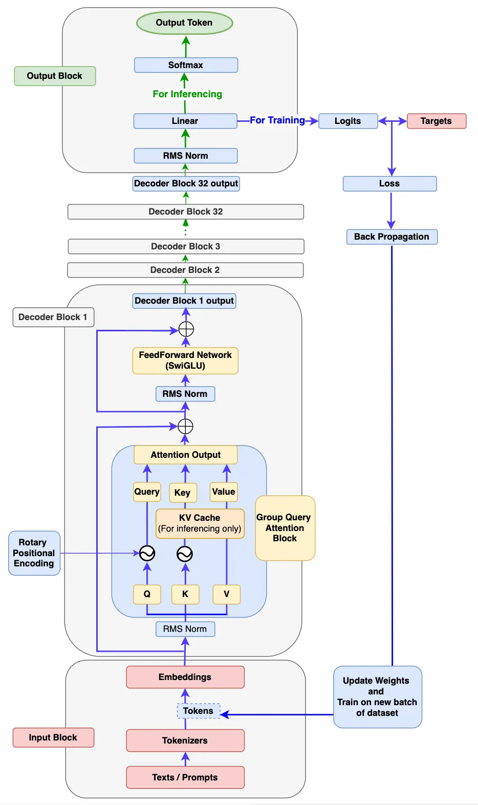
4. 使用 PyTorch 从头开始构建您自己的 Llama 3 架构

4.1 输入块

输入块有 3 个组件：文本/提示、分词器和嵌入。Input 块内部的工作流程:

• 首先, 将单个或批量的文本 / 提示传递到模型中。
• 模型的输入应始终采用数字格式, 因为它无法处理文本。Tokenizer 有助于将这些文本/提示转换为 token-ids(这是词汇表中标记的索引号表示)。我们将使用流行的 Tiny Shakespeare 数据集来构建词汇表并训练我们的模型。
• Llama 3 模型中使用的分词器是 TikToken, 一种子词分词器。但是, 我们将使用字符级分词器进行模型构建。主要原因是我们应该知道如何自己构建一个词汇表和分词器, 包括 encode 和 decode 函数。这样, 我们将能够了解后台的一切工作原理, 并且我们将完全控制代码。
• 最后, 每个token-id 将被转换为维度为 128 的嵌入向量(在原始Llama 3 8B 中, 它是4096)。然后, 嵌入将被传递到下一个名为 Decoder Block 的块中。

# Import necessary libraries
import torch
from torch import nn
from torch.nn import functional as F

import math
import numpy as np
import time
from dataclasses import dataclass
from typing import Optional, Tuple, List
import pandas as pd
from matplotlib import pyplot as plt

### Step 1: Input Block ###

# Using Tiny Shakespeare dataset for character-level tokenizer. Some part of the following character-level tokenizer is referenced from Andrej karpathy's GitHub (https://github.com/karpathy/nanoGPT/blob/master/data/shakespeare_char/prepare.py) which I found is explained very well.
# Load tiny_shakespeare data file (https://github.com/tamangmilan/llama3/blob/main/tiny_shakespeare.txt)

device: str = 'cuda' if torch.cuda.is_available() else 'cpu'   # Assign device to cuda or cpu based on availability

# Load tiny_shakespeare data file.
with open('tiny_shakespeare.txt', 'r') as f:
  data = f.read()

# Prepare vocabulary by taking all the unique characters from the tiny_shakespeare data
vocab = sorted(list(set(data)))

# Training Llama 3 model requires addtional tokens such as <|begin_of_text|>, <|end_of_text|> and <|pad_id|>, we'll add them into vocabulary
vocab.extend(['<|begin_of_text|>','<|end_of_text|>','<|pad_id|>'])
vocab_size = len(vocab)

# Create a mapping between characters with corresponding integer indexes in vocabulary.
# This is important to build tokenizers encode and decode functions.
itos = {i:ch for i, ch in enumerate(vocab)}
stoi = {ch:i for i, ch in enumerate(vocab)}

# Tokenizers encode function: take a string, output a list of integers
def encode(s):
  return [stoi[ch] for ch in s]

# Tokenizers decode function: take a list of integers, output a string
def decode(l):
  return ''.join(itos[i] for i in l)

# Define tensor token variable to be used later during model training
token_bos = torch.tensor([stoi['<|begin_of_text|>']], dtype=torch.int, device=device)
token_eos = torch.tensor([stoi['<|end_of_text|>']], dtype=torch.int, device=device)
token_pad = torch.tensor([stoi['<|pad_id|>']], dtype=torch.int, device=device)

prompts = "Hello World"
encoded_tokens = encode(prompts)
decoded_text = decode(encoded_tokens)

### Test: Input Block Code ###
# You need take out the triple quotes below to perform testing
"""
print(f"Lenth of shakespeare in character: {len(data)}")
print(f"The vocabulary looks like this: {''.join(vocab)}\n")
print(f"Vocab size: {vocab_size}")
print(f"encoded_tokens: {encoded_tokens}")
print(f"decoded_text: {decoded_text}")
"""
### Test Results: ###
"""
Lenth of shakespeare in character: 1115394
The vocabulary looks like this: 
 !$&',-.3:;?ABCDEFGHIJKLMNOPQRSTUVWXYZabcdefghijklmnopqrstuvwxyz<|begin_of_text|><|end_of_text|><|pad_id|>

Vocab size: 68
encoded_tokens: [20, 43, 50, 50, 53, 1, 35, 53, 56, 50, 42]
decoded_text: Hello World
"""

4.2 Decoder 模块

decoder 块由以下子组件组成。

4.2.1 RMS 范数(均方根归一化)

因为嵌入向量有很多维度(在 Llama3-8b 中为 4096 dim), 并且总是有可能具有不同范围内的值。这可能会导致模型梯度爆炸或消失, 从而导致收敛缓慢甚至发散。RMSNorm 将这些值引入一定范围, 这有助于稳定和加速训练过程。这使得梯度具有更一致的量级, 从而使模型收敛得更快。

为什么选择 RMSNorm 而不是图层归一化？ 说 RMSNorm 通过避免计算均值和方差来减少计算开销。此外, 根据作者的论文, RMSNorm 在不影响准确性的同时提供了性能优势。

# Step2: The Decoder Block
# Note: Since the Llama 3 model is developed by Meta, so to be in sync with their codebase and for future compatibility,
# I will use most of the code from Meta GitHub with some necessary changes required to achieve our goal.

# Define parameters dataclass: we'll use these parameters during model building, training and inference.
# Note: Since we want to see the results of training and inferencing faster rather than focusing on high accuracy, we're taking lower values for most of the parameters which are set higher in the Llama 3 model.

@dataclass
class ModelArgs:
    dim: int = 512              # embedding dimension
    n_layers: int = 8           # number of model decoder blocks
    n_heads: int = 8            # number of heads for queries embedding
    n_kv_heads: int = 4         # number of heads for keys and values embedding
    vocab_size: int = len(vocab) # Length of vocabulary
    multiple_of: int = 256        # Require to calculate dim of feedfoward network
    ffn_dim_multiplier: Optional[float] = None  # Require to calculate dim of feedfoward network
    norm_eps: float = 1e-5                       # Default Epsilon value set for the RMSNorm calculation
    rope_theta: float = 10000.0   # Default theta value for the RePE calculation

    max_batch_size: int = 10     # Max batch size
    max_seq_len: int = 256         # Max sequence length

    epochs: int = 2500             # Total number of training iteration
    log_interval: int = 10        # Number of interval to print the logs and loss values   
    device: str = 'cuda' if torch.cuda.is_available() else 'cpu'   # Assign device to cuda or cpu based on availability 

## Step2a: The RMSNorm

class RMSNorm(nn.Module):
  def __init__(self, dim: int, eps: float = 1e-6):
    super().__init__()
    device = ModelArgs.device
    self.eps = eps
    # Scaling parameter gamma, initialized with one and the no of parameters is equal to the size of dim
    self.weight = nn.Parameter(torch.ones(dim).to(device))

  def _norm(self, x):
    return x * torch.rsqrt(x.pow(2).mean(dim=-1, keepdim=True) + self.eps).to(device)

  def forward(self, x):
    #Shape: x[bs,seq,dim]
    output = self._norm(x.float()).type_as(x)

    #Shape: x[bs,seq,dim] -> x_norm[bs,seq,dim]
    return output * self.weight

### Test: RMSNorm Code ###
# You need take out the triple quotes below to perform testing
"""
x = torch.randn((ModelArgs.max_batch_size, ModelArgs.max_seq_len, ModelArgs.dim), device=device)
rms_norm = RMSNorm(dim=ModelArgs.dim)
x_norm = rms_norm(x)

print(f"Shape of x: {x.shape}")
print(f"Shape of x_norm: {x_norm.shape}")
"""
### Test Results: ###
"""
Shape of x: torch.Size([10, 256, 512])
Shape of x_norm: torch.Size([10, 256, 512])
"""

4.2.2 旋转位置编码(RoPE)

因为嵌入中没有定义模型学习的顺序。因此, 顺序对于任何语言模型都非常重要。在 Llama 3 模型架构中, RePE 用于定义句子中每个标记的位置, 不仅保持顺序, 而且保持标记在句子中的相对位置。

RoPE 是一种位置编码, 它对嵌入进行编码, 它通过添加绝对位置信息来维护句子中标记的顺序, 并在标记之间合并相对位置信息。它通过通过称为旋转矩阵的特殊矩阵旋转给定的嵌入来执行编码作。这种使用旋转矩阵的简单但非常强大的数学推导是 RoPE 的核心。

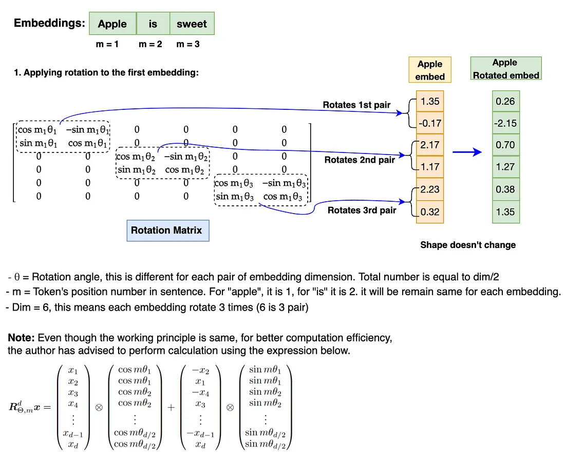
嵌入的旋转涉及每对嵌入维度的每个嵌入位置 (m) 值和 theta (θ) 的乘积。这就是 RoPE 通过实施旋转矩阵来捕获绝对位置和相对位置信息的方式。

注意：在执行旋转之前, 需要将旋转矩阵转换为极坐标形式, 并将嵌入向量转换为复数。旋转完成后, 需要将旋转的 embedding 转换回 real 以进行 attention作。此外, RoPE 仅适用于 Query 和 Key 嵌入。它不适用于 Value embedding。

## Step2b: The RoPE
def precompute_freqs_cis(dim:int, seq_len: int, theta: float=10000.0):
  # Computing Theta value for each dim pair which is dim/2
  device = ModelArgs.device
  freqs = 1.0 / (theta ** (torch.arange(0, dim, 2,device=device)[:(dim//2)].float()/dim))

  # Computing range of positions(m) in the sequence
  t = torch.arange(seq_len, dtype=torch.float32, device=device)

  # freqs gives all the Theta value range for all the position of tokens in the sequence
  freqs = torch.outer(t, freqs).to(device)

  # This is the rotation matrix which needs to be converted to Polar form in order to perform rotation to the embedding
  freqs_cis = torch.polar(torch.ones_like(freqs).to(device), freqs).to(device)
  return freqs_cis

def reshape_for_broadcast(freqs_cis, x):
  ndim = x.ndim
  assert 0<=1<ndim
  assert freqs_cis.shape == (x.shape[1],x.shape[-1]), "the last two dimension of freqs_cis, x must match"
  shape = [d if i==1 or i==ndim-1 else 1 for i,d in enumerate(x.shape)]
  return freqs_cis.view(*shape)

def apply_rotary_emb(xq: torch.Tensor, xk: torch.Tensor, freqs_cis: torch.Tensor)->Tuple[torch.Tensor, torch.Tensor]:
  device = ModelArgs.device
  # Applying rotary positional encoding to both query and key embedding together
  # First: The last dimension of xq and xk embedding needs to be reshaped to make it a pair. As rotation matrix is applied to each pair of dim.
  # Next: convert both xq and xk to complex number as the rotation matrix is only applicable to complex number
  xq_ = torch.view_as_complex(xq.float().reshape(*xq.shape[:-1], -1, 2)).to(device)    #xq_:[bsz, seq_len, n_heads, head_dim/2]
  xk_ = torch.view_as_complex(xk.float().reshape(*xk.shape[:-1], -1, 2)).to(device)    #xk_:[bsz, seq_len, n_heads, head_dim/2]

  # The rotation matrix(freqs_cis) dimensions across seq_len(dim=1) and head_dim(dim=3) should match with the embedding
  # Also, the shape freqs_cis should be the same with xq and xk, hence change the shape of freqs_cis:[seq_len,head_dim] -> freqs_cis:[1,seq_len,1,head_dim]
  freqs_cis = reshape_for_broadcast(freqs_cis, xq_)

  #Finally, perform rotation operation by multiplying with freqs_cis.
  #After the rotation is completed, convert both xq_out and xk_out back to real number and return
  xq_out = torch.view_as_real(xq_ * freqs_cis).flatten(3).to(device) #xq_out:[bsz, seq_len, n_heads, head_dim]
  xk_out = torch.view_as_real(xk_ * freqs_cis).flatten(3).to(device) #xk_out:[bsz, seq_len, n_heads, head_dim]
  return xq_out.type_as(xq), xk_out.type_as(xk)

### Test: RoPE Code ###
# Note: x_norm is calculated during RMSNorm and is being used for testing here.
# You need take out the triple quotes below to perform testing
"""
head_dim = ModelArgs.dim//ModelArgs.n_heads
wq = nn.Linear(ModelArgs.dim, ModelArgs.n_heads * head_dim, bias=False, device=device)
wk = nn.Linear(ModelArgs.dim, ModelArgs.n_kv_heads * head_dim, bias=False, device=device)
xq = wq(x_norm)
xk = wk(x_norm)
print(f"xq.shape: {xq.shape}")
print(f"xk.shape: {xk.shape}")

xq = xq.view(xq.shape[0],xq.shape[1],ModelArgs.n_heads, head_dim)
xk = xk.view(xk.shape[0],xk.shape[1],ModelArgs.n_kv_heads, head_dim)
print(f"xq.re-shape: {xq.shape}")
print(f"xk.re-shape: {xk.shape}")

freqs_cis = precompute_freqs_cis(dim=head_dim, seq_len=ModelArgs.max_seq_len)
print(f"freqs_cis.shape: {freqs_cis.shape}")

xq_rotate, xk_rotate = apply_rotary_emb(xq, xk, freqs_cis)
print(f"xq_rotate.shape: {xq_rotate.shape}")
print(f"xk_rotate.shape: {xk_rotate.shape}")
"""
### Test Results: ###
"""
xq.shape: torch.Size([10, 256, 512])
xk.shape: torch.Size([10, 256, 256])
xq.re-shape: torch.Size([10, 256, 8, 64])
xk.re-shape: torch.Size([10, 256, 4, 64])
freqs_cis.shape: torch.Size([256, 32])
xq_rotate.shape: torch.Size([10, 256, 8, 64])
xk_rotate.shape: torch.Size([10, 256, 4, 64])
"""

4.2.3 KV 缓存(仅在推理时需要)

在 Llama 3 架构中, 在推理时引入了 KV-Cache 的概念, 以 Key 和 Value 缓存的形式存储以前生成的令牌。这些缓存将用于计算自我注意以生成下一个 token。仅缓存键和值令牌, 而不缓存查询令牌, 因此称为 KV 缓存。

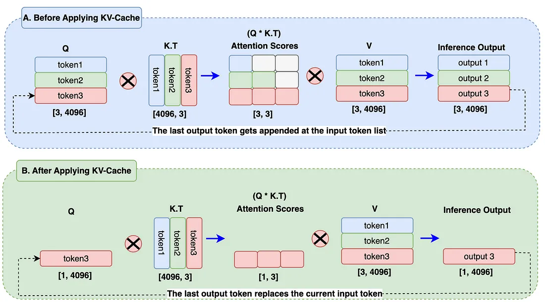
• 在图的 A 块中, 当生成 output3 标记时, 仍在计算以前的输出标记 (output1, output2), 这根本不是必需的。这导致了注意力计算过程中的额外矩阵乘法, 因此计算资源增加了很多。
• 在图的块 B 中, 输出标记替换了 Query 嵌入中的输入标记。KV Cache 存储以前生成的令牌。在注意力分数计算期间, 我们只需使用查询中的 1 个标记, 并使用 Key 和 Value 缓存中的先前标记。它将矩阵乘法从块 A 减少到 1x3 到块 B, 这几乎减少了 66%。在现实世界中, 由于序列长度和批处理大小巨大, 这将有助于显著降低计算能力。最后, 将始终只生成一个最新的输出 Token。这是引入 KV-Cache 的主要原因。

4.2.3 Group Query 分组查询注意

组查询注意力与以前的模型(如 Llama 1)中使用的 Muilt-Head 注意力相同, 唯一的区别是查询使用单独的 head, 键/值使用单独的 head。通常, 分配给 queries 的 head 数是 keys 的 n 倍, 值为 heads。让我们看一下图表以进一步建立我们的理解。

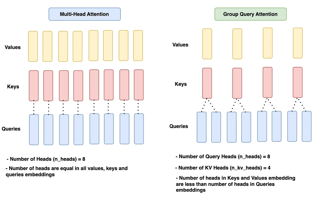
在给定的图中, 多头注意力在所有查询、键和值中具有相同数量的头, 即 n_heads = 8。

Group query attention block (组查询注意力) 块有 8 个查询头 (n_heads) 和 4 个键和值的头 (n_kv_heads), 这比查询头少 2 倍。

MultiHead Attention 已经这么好了, 为什么还需要 Group 查询 Attention呢？ 但是, 随着 KV Cache 存储的 Token 越来越多, 内存资源将显著增加。从模型性能的角度来看, 这并不是一件好事, 从财务的角度来看也是如此。因此, 引入了 Group query attention。减少 K 和 V 的磁头数量会减少要存储的参数数量, 因此使用的内存更少。各种测试结果证明, 使用这种方法, 模型精度保持在相同的范围内。

## The Attention Block [Step2c: The KV Cache; Step2d: Group Query Attention]
## As mentioned before, the naming convention follows original the meta's LLama3 GitHub

class Attention(nn.Module):
  def __init__(self, args: ModelArgs):
    super().__init__()
    self.args = args
    # Embedding dimension
    self.dim = args.dim
    # Number of heads assigned to Query
    self.n_heads = args.n_heads
    # Number of heads assigned to Key and values. If "None", the number will be same as Query.
    self.n_kv_heads = args.n_heads if args.n_kv_heads is None else args.n_kv_heads
    # Dimension of each head relative to model dimension
    self.head_dim = args.dim // args.n_heads
    # Number of repetition in order to make time Key, Value heads to match Query heads number
    self.n_rep = args.n_heads // args.n_kv_heads

    # Weight initialize for Keys, Querys, Values and Oupt. Notice that the out_feature value of weight for q and kv are based on it's heads
    self.wq = nn.Linear(self.dim, self.n_heads * self.head_dim, bias=False, device=device)
    self.wk = nn.Linear(self.dim, self.n_kv_heads * self.head_dim, bias=False, device=device)
    self.wv = nn.Linear(self.dim, self.n_kv_heads * self.head_dim, bias=False, device=device)
    self.wo = nn.Linear(self.n_heads * self.head_dim, self.dim, bias=False, device=device)

    # Initialize caches to store Key, Values at start. (KV Cache Implementation)
    self.cache_k = torch.zeros((args.max_batch_size, args.max_seq_len, self.n_kv_heads, self.head_dim), device=args.device)
    self.cache_v = torch.zeros((args.max_batch_size, args.max_seq_len, self.n_kv_heads, self.head_dim), device=args.device)

  def forward(self, x: torch.Tensor, start_pos, inference):
    # Shape of the input embedding: [bsz,seq_len,dim]
    bsz, seq_len, _ = x.shape
    # Mask will be used during 'Training' and is not required for 'inference' due to the use of KV cache.
    mask = None

    xq = self.wq(x)  #x[bsz,seq_len,dim]*wq[dim,n_heads * head_dim] -> q[bsz,seq_len,n_heads * head_dim]
    xk = self.wk(x)  #x[bsz,seq_len,dim]*wq[dim,n_kv_heads * head_dim] -> k[bsz,seq_len,n_kv_heads * head_dim]
    xv = self.wv(x)  #x[bsz,seq_len,dim]*wq[dim,n_kv_heads * head_dim] -> v[bsz,seq_len,n_kv_heads * head_dim]

    # Reshaping Querys, Keys and Values by their number of heads. (Group Query Attention Implementation)
    xq = xq.view(bsz, seq_len, self.n_heads, self.head_dim)      #xq[bsz,seq_len,n_heads, head_dim]
    xk = xk.view(bsz, seq_len, self.n_kv_heads, self.head_dim)   #xk[bsz,seq_len,n_kv_heads, head_dim]
    xv = xv.view(bsz, seq_len, self.n_kv_heads, self.head_dim)   #xv[bsz,seq_len,n_kv_heads, head_dim]

    # Model - Inference Mode: kv-cache is enabled at inference mode only.
    if inference:
      # Compute rotation matrix for each position in the sequence
      freqs_cis = precompute_freqs_cis(dim=self.head_dim, seq_len=self.args.max_seq_len * 2)
      # During inferencing, we should only take the rotation matrix range from the current position of the tokens.
      freqs_cis = freqs_cis[start_pos : start_pos + seq_len]
      # Apply RoPE to Queries and Keys embeddings
      xq, xk = apply_rotary_emb(xq, xk, freqs_cis)

      self.cache_k = self.cache_k.to(xq)
      self.cache_v = self.cache_v.to(xq)
      # Store Keys and Values token embedding into their respective cache [KV Cache Implementation]
      self.cache_k[:bsz, start_pos:start_pos + seq_len] = xk
      self.cache_v[:bsz, start_pos:start_pos + seq_len] = xv

      # Assign all the previous tokens embeddings upto current tokens position to Keys and Values variable for Attention Calculation
      keys = self.cache_k[:bsz, :start_pos + seq_len]
      values = self.cache_v[:bsz, :start_pos + seq_len]

      # At this point, they Keys and Values shape aren't same with Queries Embedding which has to be in order to computer attention score
      # Use repeat_kv function to make Keys,Values shape same as queries shape
      keys = repeat_kv(keys, self.n_rep)      #keys[bsz,seq_len,n_heads,head_dim]
      values = repeat_kv(values, self.n_rep)  #values[bsz,seq_len,n_heads,head_dim]

    # Mode - Training mode: KV-Cache not implemented
    else:
      # Compute rotation matrix and apply RoPE to queries and keys for for training.
      freqs_cis = precompute_freqs_cis(dim=self.head_dim, seq_len=self.args.max_seq_len)

      #xq[bsz,seq_len,n_heads, head_dim], xk[bsz,seq_len,n_heads, head_dim]
      xq, xk = apply_rotary_emb(xq, xk, freqs_cis)

      # Use repeat_kv function to make Keys,Values shape same as the queries shape
      #keys[bsz,seq_len,n_heads,head_dim], #values[bsz,seq_len,n_heads,head_dim]
      keys = repeat_kv(xk, self.n_rep)
      values = repeat_kv(xv, self.n_rep)

      # For training mode, we'll compute mask and apply to the attention score later
      mask = torch.full((seq_len, seq_len),float("-inf"),device=self.args.device)
      mask = torch.triu(mask, diagonal=1).to(self.args.device)

    # To compute attention, we'll need to perform a transpose operation to reshape all queries, keys and values bring heads at dim 1 and seq at dim 2
    xq = xq.transpose(1,2)                  #xq[bsz,n_heads,seq_len,head_dim]
    keys = keys.transpose(1,2)              #keys[bsz,n_heads,seq_len,head_dim]
    values = values.transpose(1,2)          #values[bsz,n_heads,seq_len,head_dim]

    # Computing attention score
    scores = torch.matmul(xq, keys.transpose(2,3)).to(self.args.device)/math.sqrt(self.head_dim)
    if mask is not None:
      scores = scores + mask

    # Apply softmax to the attention score
    scores = F.softmax(scores.float(), dim=-1).type_as(xq)
    # Matrix multiplication of attention score with the values
    output = torch.matmul(scores, values).to(self.args.device)

    # We get the contextual embedding for each head
    # All heads need to be reshaped back and combined to give a single single contextual attention output
    # Shape change: output[bsz,n_heads,seq_len,head_dim] -> output[bsz,seq_len, n_heads,head_dim] -> output[bsz,seq_len, n_heads * head_dim]
    output = output.transpose(1,2).contiguous().view(bsz, seq_len, -1)

    # shape: output [bsz,seq_len,dim]
    return self.wo(output)

# If the number of keys/values heads is less than query heads, this function expands the key/values embeddings with the required number of repetition
def repeat_kv(x:torch.Tensor, n_rep: int)-> torch.Tensor:
  bsz, seq_len, n_kv_heads, head_dim = x.shape
  if n_rep == 1:
    return x
  return (
      x[:,:,:,None,:]
      .expand(bsz,seq_len,n_kv_heads,n_rep, head_dim)
      .reshape(bsz,seq_len,n_kv_heads * n_rep, head_dim)
  )


### Test: Repeat_kv function ###
# note: xk, x_norm is already calculated during RoPE, RMSNorm testing and is being used for testing here.
# You need take out the triple quotes below to perform testing
"""
n_rep = ModelArgs.n_heads // ModelArgs.n_kv_heads
keys = repeat_kv(xk, n_rep)
print(f"xk.shape: {xk.shape}")
print(f"keys.shape: {keys.shape}")

## Test: Attention function
# You need take out the triple quotes below to perform testing

attention = Attention(ModelArgs)
x_out = attention(x_norm,start_pos=0, inference=False)
print(f"x_out.shape: {x_out.shape}")
"""
### Test Results: ###
"""
xk.shape: torch.Size([10, 256, 4, 64])
keys.shape: torch.Size([10, 256, 8, 64])
x_out.shape: torch.Size([10, 256, 512])
"""

4.2.4 FeedForward 网络(SwiGLU 激活)

注意力输出首先在 RMSNorm 期间被规范化, 然后馈送到 FeedForward 网络。在前馈网络内部, 注意力输出嵌入将在其隐藏层中扩展到更高的维度, 并学习令牌的更复杂的特征。

为什么使用 SwiGLU 而不是 ReLU？

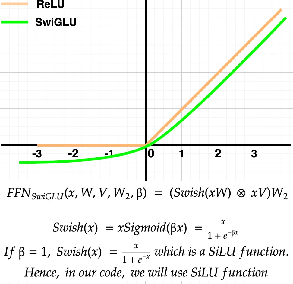
如上图所示, SwiGLU 函数在正轴上的行为几乎与 ReLU 相似。但是, 在负轴上, SwiGLU 会输出一些负值, 这在学习更小而不是在 ReLU 的情况下是平坦的 0 时可能很有用。总体而言, 根据作者的说法, SwiGLU 的性能优于 ReLU;因此, 它被选中了。

## Step2e: The Feedfoward Network (SwiGLU activation)
class FeedForward(nn.Module):
  def __init__(self, dim:int, hidden_dim:int, multiple_of:int, ffn_dim_multiplier: Optional[float]):
    super().__init__()
    # Models embedding dimension
    self.dim = dim

    # We must use the hidden dimensions calculation shared by Meta which is the ideal one for this model
    # Hidden dimension are calculated such that it is a multiple of 256.
    hidden_dim = int(2 * hidden_dim/3)
    if ffn_dim_multiplier is not None:
      hidden_dim = int(ffn_dim_multiplier * hidden_dim)
    hidden_dim = multiple_of * ((hidden_dim + multiple_of - 1) // multiple_of)

    # define hiddne layers weights
    self.w1 = nn.Linear(self.dim, hidden_dim, bias=False, device=device)
    self.w2 = nn.Linear(hidden_dim, self.dim, bias=False, device=device)
    self.w3 = nn.Linear(self.dim, hidden_dim, bias=False, device=device)

  def forward(self, x):
    # Shape: [bsz,seq_len,dim]
    return self.w2(F.silu(self.w1(x)) * self.w3(x))



### Test: FeedForward module ###
# note: x_out is already computed at Attention testing and is being used for testing here.
# You need take out the triple quotes below to perform testing
"""
feed_forward = FeedForward(ModelArgs.dim, 4 * ModelArgs.dim, ModelArgs.multiple_of, ModelArgs.ffn_dim_multiplier)
x_out = rms_norm(x_out)
x_out = feed_forward(x_out)
print(f"feed forward output: x_out.shape: {x_out.shape}")
"""

### Test Results: ###
"""
feed forward output: x_out.shape: torch.Size([10, 256, 512])
"""

4.2.5 Decoder 块

• 来自 input 块的 embedding 被馈送到 Attention-RMSNorm 块中。这将进一步馈送到 Group Query Attention 块中。
• 然后, 来自 input 块的相同 embedding 将被添加到 attention 输出中。
• 之后, 注意力输出被馈送到 FeedFoward-RMSNorm 中, 并进一步被馈送到 FeedFoward 网络块中。
• 然后, FeedFoward 网络的输出将再次添加 attention 输出。
• 生成的输出称为 Decoder Output。 然后, 此 decoder output 作为 input 馈送到另一个 decoder 块中。对于接下来的 31 个 decoder 块, 将重复相同的作。然后, 第 32 个 decoder 模块的最终 decoder 输出将传递到 Output 模块。

## Step2f: The Decoder Block. The class name is assigned as TransformerBlock to match the name of Meta llama 3 code base.

class TransformerBlock(nn.Module):
  def __init__(self, args: ModelArgs):
    super().__init__()
    self.args = args
    # Initilizate RMSNorm for attention
    self.attention_norm = RMSNorm(dim=args.dim, eps = args.norm_eps)
    # Initilizate Attention class
    self.attention = Attention(args)
    # Initilizate RMSNorm for feedfoward class
    self.ff_norm = RMSNorm(dim=args.dim, eps = args.norm_eps)
    # Initilizate feedfoward class
    self.feedforward = FeedForward(args.dim, 4 * args.dim, args.multiple_of, args.ffn_dim_multiplier)

  def forward(self, x, start_pos, inference):
    # start_pos = token position for inference mode, inference = True for inference and False for training mode
    # i) pass input embedding to attention_norm and then pass to attention block.
    # ii) the output of attention is then added to embedding(before norm)
    h = x + self.attention(self.attention_norm(x), start_pos, inference)

    # i) pass attention output to ff_norm and then pass to the feedforward network.
    # ii) the output of feedforward network is then added to the attention output(before ff_norm)
    out = h + self.feedforward(self.ff_norm(h))
    # Shape: [bsz,seq_len,dim]
    return out


### Test: TransformerBlock ###
# You need take out the triple quotes below to perform testing
"""
x = torch.randn((ModelArgs.max_batch_size, ModelArgs.max_seq_len, ModelArgs.dim), device=device)
transformer_block = TransformerBlock(ModelArgs)
transformer_block_out = transformer_block(x,start_pos=0, inference=False)
print(f"transformer_block_out.shape: {transformer_block_out.shape}")
"""

### Test Results: ###
"""
transformer_block_out.shape: torch.Size([10, 64, 128])
"""

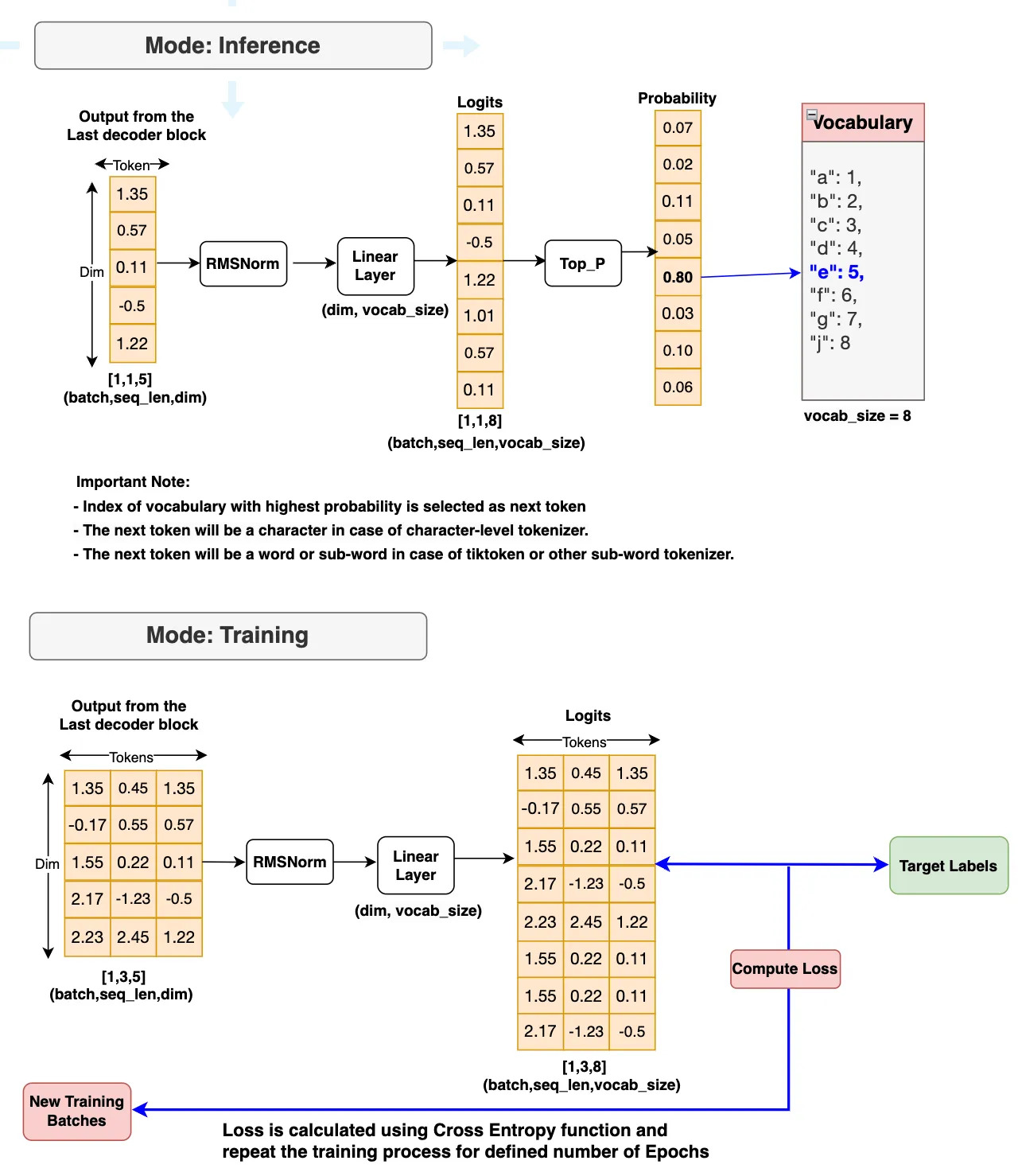
4.3 输出块

最终 decoder block 的 decoder output 将馈送到 output block 中。它首先被馈送到 RMSNorm 中。然后, 它将馈送到生成 logit 的线性层。接下来, 将发生以下两个作之一。

• 如果模式为 inference, 则计算top_p概率并生成下一个标记。如果达到最大生成长度或将句尾标记生成为下一个标记, 则生成的下一个标记将停止。
• 如果模式为 Training, 则使用目标标签计算损失, 并重复训练, 直到达到最大纪元长度。

最后, 让我们组合 3 个模块(输入模块、解码器模块和输出模块)的所有组件。这就给出了我们最终的 Llama 3 模型。

## Step3: The Output Block
# This is the Llama 3 model. Again, the class name is maintained as Transformer to match with Meta Llama 3 model.

class Transformer(nn.Module):
  def __init__(self, params: ModelArgs):
    super().__init__()
    # set all the ModelArgs in params variable
    self.params = params
    # Initilizate embedding class from the input block
    self.tok_embeddings = nn.Embedding(params.vocab_size, params.dim)

    # Initialize the decoder block and store it inside the ModuleList. 
    # This is because we've 4 decoder blocks in our Llama 3 model. (Official Llama 3 has 32 blocks)
    self.layers = nn.ModuleList()
    for layer_id in range(params.n_layers):
      self.layers.append(TransformerBlock(args=params))

    # Initilizate RMSNorm for the output block
    self.norm = RMSNorm(params.dim, eps = params.norm_eps)
    
    # Initilizate linear layer at the output block.
    self.output = nn.Linear(params.dim, params.vocab_size, bias=False)

  def forward(self, x, start_pos=0, targets=None):
    
    # start_pos = token position for inference mode, inference = True for inference and False for training mode
    # x is the batch of token_ids generated from the texts or prompts using tokenizers.
    # x[bsz, seq_len] -> h[bsz, seq_len, dim]
    h = self.tok_embeddings(x)

    # If the target is none, Inference mode is activated and set to "True" and "False" if Training mode is activated.
    if targets is None:
      inference = True
    else:
      inference = False

    # The embeddings (h) will then pass though all the decoder blocks.
    for layer in self.layers:
      h = layer(h, start_pos, inference)

    # The output from the final decoder block will feed into the RMSNorm
    h = self.norm(h)

    # After normalized, the embedding h will then feed into the Linear layer. 
    # The main task of the Linear layer is to generate logits that maps the embeddings with the vocabulary size.
    # h[bsz, seq_len, dim] -> logits[bsz, seq_len, vocab_size]
    logits = self.output(h).float()
    loss = None

    # Inference mode is activated if the targets is not available
    if targets is None:
      loss = None
    # Training mode is activated if the targets are available. And Loss will be calculated for further model training. 
    else:
      loss = F.cross_entropy(logits.view(-1, self.params.vocab_size), targets.view(-1))

    return logits, loss


### Test: Transformer (Llama Model) ###
# You need take out the triple quotes below to perform testing
"""
model = Transformer(ModelArgs).to(ModelArgs.device)
print(model)
"""

4.4 训练我们的 Llama 3 模型

## Step 4: Train Llama 3 Model:

# Create a dataset by encoding the entire tiny_shakespeare data token_ids list using the tokenizer's encode function that we've built at the input block section
dataset = torch.tensor(encode(data), dtype=torch.int).to(ModelArgs.device)
print(f"dataset-shape: {dataset.shape}")

# Define function to generate batches from the given dataset
def get_dataset_batch(data, split, args:ModelArgs):
  seq_len = args.max_seq_len
  batch_size = args.max_batch_size
  device = args.device

  train = data[:int(0.8 * len(data))]
  val = data[int(0.8 * len(data)): int(0.9 * len(data))]
  test = data[int(0.9 * len(data)):]

  batch_data = train
  if split == "val":
    batch_data = val

  if split == "test":
    batch_data = test
  
  # Picking random starting points from the dataset to give random samples for training, validation and testing.
  
  ix = torch.randint(0, len(batch_data) - seq_len - 3, (batch_size,)).to(device)
  x = torch.stack([torch.cat([token_bos, batch_data[i:i+seq_len-1]]) for i in ix]).long().to(device)
  y = torch.stack([torch.cat([batch_data[i+1:i+seq_len], token_eos]) for i in ix]).long().to(device)
  
  return x,y

### Test: get_dataset function ###
"""
xs, ys = get_dataset_batch(dataset, split="train", args=ModelArgs)
print([(decode(xs[i].tolist()), decode(ys[i].tolist())) for i in range(len(xs))])
"""

# Define a evaluate loss function to calculate and store training and validation loss for logging and plotting
@torch.no_grad()
def evaluate_loss(model, args:ModelArgs):
  out = {}
  model.eval()

  for split in ["train", "val"]:
    losses = []
    for _ in range(10):      
      xb, yb = get_dataset_batch(dataset, split, args)
      _, loss = model(x=xb, targets=yb)
      losses.append(loss.item())
    out[split] = np.mean(losses)

  model.train()
  return out

# Define a training function to perform model training
def train(model, optimizer, args:ModelArgs):
    epochs = args.epochs
    log_interval = args.log_interval
    device = args.device
    losses = []   
    start_time = time.time()

    for epoch in range(epochs):
        optimizer.zero_grad()
        
        xs, ys = get_dataset_batch(dataset, 'train', args)
        xs = xs.to(device)
        ys = ys.to(device)
        logits, loss = model(x=xs, targets=ys)
        loss.backward()
        optimizer.step()

        if epoch % log_interval == 0:
            batch_time = time.time() - start_time
            x = evaluate_loss(model, args)
            losses += [x]            
            print(f"Epoch {epoch} | val loss {x['val']:.3f} | Time {batch_time:.3f}")
            start_time = time.time()
    
    # Print the final validation loss
    print("validation loss: ", losses[-1]['val'])
    # Display the interval losses in plot 
    return pd.DataFrame(losses).plot()

从下面的代码块开始训练, 训练完成后观察图中的训练结果。

## Start training our Llama 3 model
model = Transformer(ModelArgs).to(ModelArgs.device)
optimizer = torch.optim.Adam(model.parameters())

train(model, optimizer, ModelArgs)

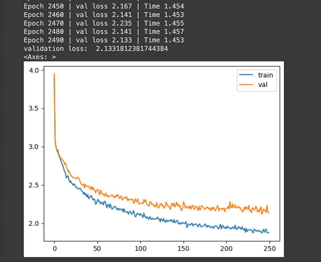
上图显示了训练和验证损失图。该培训已经进行了 2500 多个时期。使用默认 GPU 和 RAM 设置的 Google Colab 完成训练过程大约需要 10 分钟, 这非常快。最终 epoch 的验证损失为 2.19, 考虑到我们使用的训练数据量和 epoch 的数量, 这被认为是可以的。为了显着减少损失, 我们将不得不增加训练数据的大小、更多的 epoch 数和更高的 GPU 或处理能力。

4.5 推理 Llama 3 模型

## Step 5: Inference Llama 3 Model:
# This function generates text sequences based on provided prompts using the LLama 3 model we've built and trained.

def generate(model, prompts: str, params: ModelArgs, max_gen_len: int=500, temperature: float = 0.6, top_p: float = 0.9):

    # prompt_tokens: List of user input texts or prompts
    # max_gen_len: Maximum length of the generated text sequence.
    # temperature: Temperature value for controlling randomness in sampling. Defaults to 0.6.
    # top_p: Top-p probability threshold for sampling prob output from the logits. Defaults to 0.9.
    # prompt_tokens = [0]
    bsz = 1  #For inferencing, in general user just input one prompt which we'll take it as 1-batch
    prompt_tokens = token_bos.tolist() + encode(prompts)
    assert len(prompt_tokens) <= params.max_seq_len, "prompt token length should be small than max_seq_len"
    total_len = min(len(prompt_tokens)+max_gen_len, params.max_seq_len)   

    # this tokens matrix is to store the input prompts and all the output that is generated by model.
    # later we'll use the tokenizers decode function to decode this token to view results in text format
    tokens = torch.full((bsz,total_len), fill_value=token_pad.item(), dtype=torch.long, device=params.device)

    # fill in the prompt tokens into the token matrix
    tokens[:,:len(prompt_tokens)] = torch.tensor(prompt_tokens, dtype=torch.long, device=params.device)

    #create a prompt_mask_token for later use to identify if the token is a prompt token or a padding token
    # True if it is a prompt token, False if it is a padding token
    input_text_mask = tokens != token_pad.item()

    #now we can start inferencing using one token at a time from the prompt_tokens list starting with the first position.
    prev_pos = 0
    for cur_pos in range(1, total_len):
      with torch.no_grad():
        logits, _ = model(x=tokens[:,prev_pos:cur_pos], start_pos=prev_pos)
      if temperature > 0:      
        probs = torch.softmax(logits[:, -1]/temperature, dim=-1)
        next_token = sample_top_p(probs, top_p)        
      else:
        next_token = torch.argmax(logits[:, -1], dim=-1)        

      next_token = next_token.reshape(-1)

      # only replace the token if it's a padding token
      next_token = torch.where(input_text_mask[:, cur_pos], tokens[:, cur_pos], next_token)
      tokens[:, cur_pos] = next_token

      prev_pos = cur_pos
      if tokens[:,cur_pos]==token_pad.item() and next_token == token_eos.item():
        break

    output_tokens, output_texts = [], []    

    for i, toks in enumerate(tokens.tolist()):
      # eos_idx = toks.index(token_eos.item())
      if token_eos.item() in toks:
        eos_idx = toks.index(token_eos.item())
        toks = toks[:eos_idx]

      output_tokens.append(toks)
      output_texts.append(decode(toks))
    return output_tokens, output_texts

# Perform top-p (nucleus) sampling on a probability distribution.
# probs (torch.Tensor): Probability distribution tensor derived from the logits.
# p: Probability threshold for top-p sampling.
# According to the paper, Top-p sampling selects the smallest set of tokens whose cumulative probability mass exceeds the threshold p. 
# The distribution is renormalized based on the selected tokens.
def sample_top_p(probs, p):
    probs_sort, prob_idx = torch.sort(probs, dim=-1, descending=True)
    probs_sum = torch.cumsum(probs_sort, dim=-1)
    mask = probs_sum - probs_sort > p
    probs_sort[mask] = 0.0
    probs_sort.div_(probs_sort.sum(dim=-1, keepdim=True))
    next_token = torch.multinomial(probs_sort, num_samples=1)
    next_token = torch.gather(prob_idx, -1, next_token)    
    # Sampled token indices from the vocabular is returned 
    return next_token

对新的 Prompts 执行推理并检查生成的输出

## Perform the inferencing on user input prompts
prompts = "Consider you what services he has done"
output_tokens, output_texts = generate(model, prompts, ModelArgs)
output_texts = output_texts[0].replace("<|begin_of_text|>", "")
print(output_texts)

## Output ##
"""
Consider you what services he has done o eretrane
adetranytnn i eey i ade hs rcuh i eey,ad hsatsTns rpae,T
eon o i hseflns o i eee ee hs ote i ocal ersl,Bnnlnface
o i hmr a il nwye ademto nt i a ere
h i ees.
Frm oe o etrane o oregae,alh,t orede i oeral
"""

参考:

https://github.com/facebookresearch/llama
https://github.com/soulteary/llama-docker-playground
https://github.com/markasoftware/llama-cpu
https://writesonic.com/blog/chatgpt-prompts/#chatgpt-prompts-for-content
Build Your Own Llama 3 Architecture from Scratch Using PyTorch